Deep dive to unravel the mystery of Neural Networks, stepping outside the theoretical boundaries.

A lot has been said and written about Neural Networks (NNs) in recent years — right from the concept of Perceptron to the complex Multilayer Architecture of Neurons. This article is an attempt to demystify the two fundamental algorithms, Feed-forward and Back-propagation, that enable the working of a Neural Network. These techniques have been explained in their simplest form using Microsoft Excel.

The example taken into consideration is really basic and far from the real-world example. The intention here is to keep it simple and intuitive, to understand the working logic, rather than focusing on the complex mathematics behind it.

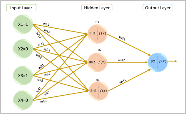
To begin with, I have considered just one input vector V= [X1=1, X2= 0, X3=1, X4=0] with a single hidden layer consisting of 3 neurons and an output layer. The target output is 1.

Neural Network with One Hidden Layer

Network set up-

Input and Output- As an example, let us say we expect the algorithm to give an output of ‘1’ for an indicated non-zero value for ‘X1’ & ‘X3’ (say, 1) and zero for ‘X2’ & ‘X4’. So, the input vector considered here is [1,0,1,0].

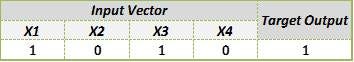
Input and Output

Feed-forward:

Step 1: Initialize network parameters

First step is to initialize weights and biases using rand() function in MS Excel.

(P.S: The highlighted cells in all tables below represent derived values based on the suggested formulae)

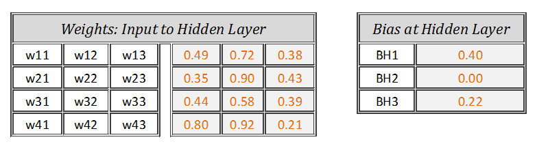
Weights and Biases — Input to Hidden Layer

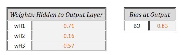
Weights and Biases — Hidden to Output Layer

Step 2: Calculate Net Input at hidden layer nodes

Net Input is nothing but input multiplied by weight, then incremented by bias. Using matrix multiplication of input vector [1x4] and weights [4x3], the resultant matrix is of dimension [1X3]. To get this working in excel, use \=SUMPRODUCT() to arrive at resultant matrix [1X3] as below-

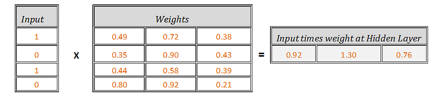
Input times Weight

Now, add biases to these Input times weight,

Net Input

Step 3: Pass the Net Inputs through the activation function (Sigmoid)

Let’s pass the output from ‘Step 2’ [1.33,1.30,0.99] as input to the activation function at each neuron of hidden layer as [f(1.33),f(1.30),f(0.99)], which can easily be done by f(x) = 1/(1+exp (-x)) .

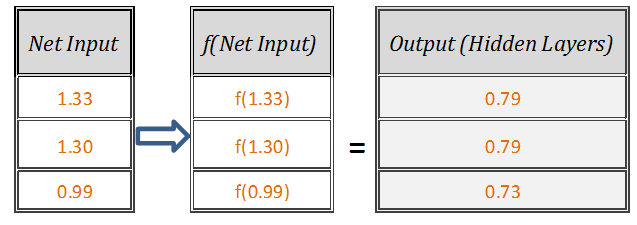
Output at Hidden Layer

Step 4: Calculate Net Input at output node

Now the outputs from ‘Step 3’ [0.79,0.79,0.73] will act as inputs to the output node. Let’s repeat ‘Step 2’ with input vector as [0.79,0.79,0.73], weight vector as [0.71,0.16,0.57] and output bias as[0.83].

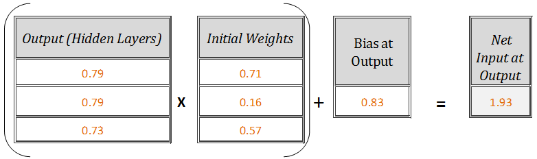
Net Input at Output Node

which after simplification = 1.93

Step 5: Obtain final output of neural network

Let’s pass the output received from ‘Step 4’ [1.93] to the activation function as f(1.93), which again can be calculated using f(x)=1/(1+exp(-x)), thus resulting in the final output of neural network.

\=1/(1+exp(-1.93))

Feed-forward Network Output =0.87

Back-propagation:

Once the output from Feed-forward is obtained, the next step is to assess the output received from the network by comparing it with the target outcome.

Now, one obvious thing that’s in control of the NN designer are the weights and biases (also called parameters of network). So, the challenge here is to find the optimal weights and biases that can minimise the sum of square error: E=1/2 ∑ (Network output-Target output)² received by the network, which in this case = [0.5*(-0.13)²] = 0.00798

We need to look at the error contributed by each of these weights and biases individually and then keep updating them accordingly to reduce the error. This process will be iterated till the convergence. The network will be called a trained network once an optimal is reached. Let’s start implementing this theory in Excel.

Step 1: Update weights [wH1, wH2, wH3]

Calculate derivative of error function E with respect to weights [wH1, wH2, wH3] using chain rule (I’ll skip the derivation here), which after simplification is equal to the product of

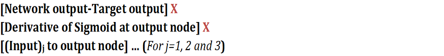
where, Derivative of sigmoid function f(x) = [f(x)\(1-f(x)]*

So, [d(E)/d(wH1), d(E)/d(wH2), d(E)/d(wH3)] =

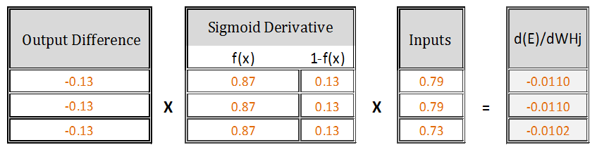
Derivative of E with respect to WH1, WH2 and WH3 respectively

The new updated weights will be [Initial weights] — [{(learning rate)* [d(E)/d(wH1), d(E)/d(wH2), d(E)/d(wH3)]}], where, learning rate is assumed to be 0.5

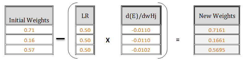
Updated weights after 1st Iteration

Step 2 — Update bias BO at Output node

For bias, calculate the derivative of error function E with respect to bias BO using chain rule, which after simplification is equal to the product of

So, d(E)/d(BO)=

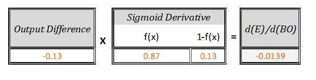
Derivative of Error E with respect to output node bias

New updated Bias [BO]new = [Initial Bias] — [learning rate *{d(E)/d(BO)}]

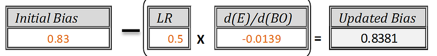
Update Bias at Output node after 1st Iteration

Step 3- Update weights [w11, w12, ……w43]

To update weights at “Input to Hidden” layer, let’s calculate derivative of error E with respect to weights [W11, W12….W43] which after simplification is equal to the product of

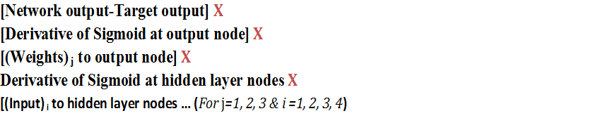
So, [d(E)/d(w11), d(E)/d(w12),……d(E)/d(w43)] =

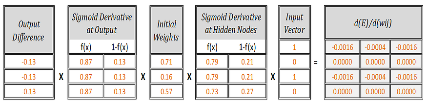
Derivatives of error E with respect to weights w11, w12,….w43

New updated weights = [Initial weights] — [learning rate * (d(E)/dwij)]

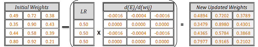
Updated Weight after 1st Iteration

Excel formula to be used to update the weights

Step 4: Update the bias [BH1,BH2,BH3]

Same way, calculate derivative of error E with respect to the biases at hidden node using chain rule, which after simplification is equal to the product of

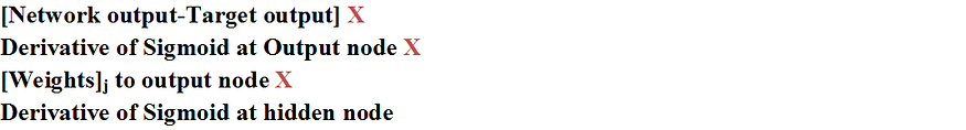
So, [d(E)/d(BH1), d(E)/d(BH2), d(E)/d(BH3)] =

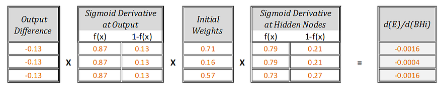
Derivative of error E with respect to Bias at Hidden nodes

New updated biases = [Initial bias] — [learning rate * (d(E)/d(BHi))]

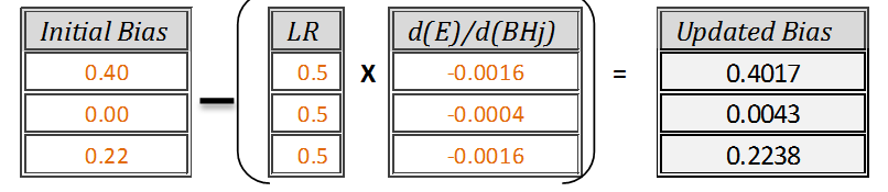
Updated Hidden node Bias after 1st Iteration

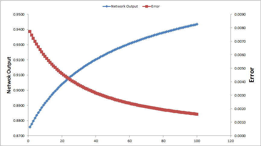
Thus, we have completed one loop of Feed-forward and Back-propagation, Repetition of the same steps i.e. running Feed-forward again with these updated parameters will take you one step closer to the target output and once again, Back-propagation will be used to update these parameters. This cyclic process of Feed-forward and Back-Propagation will continue till the error becomes almost constant and there is not much scope of further improvement in target output.

After 100 iterations shows the behaviour of the network as below. With each iteration, Network Output progresses towards the target output (Blue Line) with reduction in error (Red Line).

Note: This blog is reproduced from the Gaurav Gupta blog.